Example Project: A discrete solution to the time-dependent Schrodinger equation

The complex problem solved in this example group project is: How can we model quantum tunneling through a finite barrier?

Roughly the outline of this project goes like this:

1. Set up equations needed to solve this problem
2. Determine boundary and initial conditions needed
3. Set up the system of equations in matrix form, and solve
4. Visualize solution
5. Explain the computing tool of choice: numpy arrays

Part 1: Setup of equations

Quantum tunneling can be measured if we know the probability that a wavefunction passes through the barrier. This is a matter of using the wavefunction to compute probability density: $f(x, t) = |\psi(x, t)|^2$. We can solve for wavefunction values at different times and positions using Schrodinger's equation, which we can discretize using finite difference methods.

Schrodinger's Equation:

$$-\frac{\hbar}{2m} \frac{\partial^2\psi}{\partial x^2} + V(x)\psi = i\hbar \frac{\partial\psi}{\partial t} $$

Finite difference methods:

$$\frac{dy_i}{dx} = \frac{y_{i+1}-y_{i-1}}{2h}$$

$$\frac{d^2 y_i}{dx^2} = \frac{y_{i-1}-2y_i+y_{i+1}}{h^2}$$

Combining these, we get:

$$-\frac{\hbar}{2m} \left( \frac{\psi(x_{i-1}, t_j)-2\psi(x_i, t_j)+\psi(x_{i+1}, t_j)}{\Delta x^2}\right) + V(x_i)\psi(x_i, t_j) = i\hbar\frac{\psi(x_i, t_{j+1})-\psi(x_i, t_{j-1})}{2\Delta t} $$

We can split into real and imaginary components to get rid any complex numbers and also clear up any potential confusion with the two meanings of "$i$" in the equation above. We can use $\psi_{i,j}$ as shorthand for $\psi(x_i, t_j)$. We begin by defining $\psi^{(R)}$ and $\psi^{(I)}$, the real and imaginary components of the wavefunction.

$$\psi_{i,j} = \psi^{(R)}_{i,j} + i \psi^{(I)}_{i,j}$$

$$-\frac{\hbar}{2m} \left( \frac{\psi^{(R)}_{i-1,j}-2\psi^{(R)}_{i,j}+\psi^{(R)}_{i+1,j}}{\Delta x^2}\right) + V_i\psi^{(R)}_{i,j} = -\hbar\frac{\psi^{(I)}_{i,j+1}-\psi^{(I)}_{i,j-1}}{2\Delta t} $$

$$-\frac{\hbar}{2m} \left( \frac{\psi^{(I)}_{i-1,j}-2\psi^{(I)}_{i,j}+\psi^{(I)}_{i+1,j}}{\Delta x^2}\right) + V_i\psi^{(I)}_{i,j} = \hbar\frac{\psi^{(R)}_{i,j+1}-\psi^{(R)}_{i,j-1}}{2\Delta t} $$

One final issue with this equations is that the times on the right-hand-side span $j-1$ to $j+1$. This is total of three time steps! To reduce the time span in a single equation, and make it possible to incrementally calculate values of the wavefunction from one time-value to the next, we can use $\Delta t / 2$ time steps in these equations.

What this means practically is that the right-hand-side would have time values spanning from $j$ to $j+1$, or $j-1/2$ to $j+1/2$. We start by rewriting the first equation in this way:

$$-\frac{\hbar}{2m} \left( \frac{\psi^{(R)}_{i-1,j}-2\psi^{(R)}_{i,j}+\psi^{(R)}_{i+1,j}}{\Delta x^2}\right) + V_i\psi^{(R)}_{i,j} = -\hbar\frac{\psi^{(I)}_{i,j+1/2}-\psi^{(I)}_{i,j-1/2}}{\Delta t} $$

The time represented here is still centered on $j$, but now we have used terms like $\psi^{(I)}_{i,j-1/2}$ and $\psi^{(I)}_{i,j+1/2}$. This means we are now counting the imaginary part of the wavefunction using times staggered by a half-time-step. This necessitates a change in the second equation to reflect this new paradigm:

$$-\frac{\hbar}{2m} \left( \frac{\psi^{(I)}_{i-1,j+1/2}-2\psi^{(I)}_{i,j+1/2}+\psi^{(I)}_{i+1,j+1/2}}{\Delta x^2}\right) + V_i\psi^{(I)}_{i,j} = \hbar\frac{\psi^{(R)}_{i,j+1}-\psi^{(R)}_{i,j}}{\Delta t} $$

And with that, we solved the time span issue! However, this now means we will be solving for $\psi^{(R)}_{i,j}$ and $\psi^{(I)}_{i,j+1/2}$.

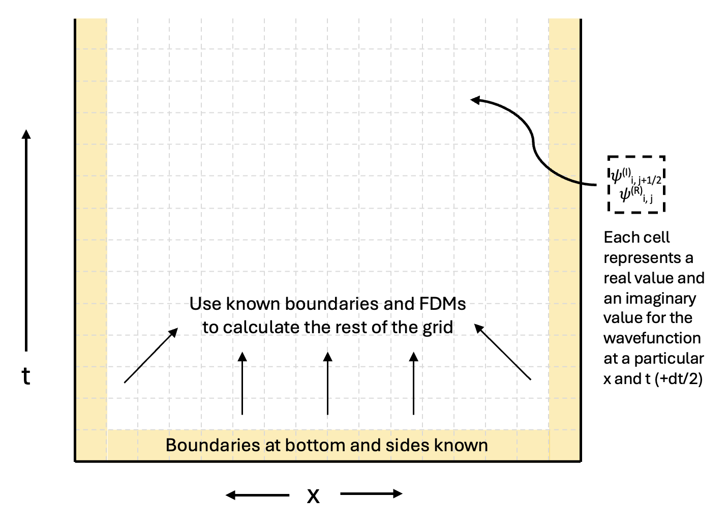
We can set up a 2D grid of $\psi$ values. Left/right is x-direction, and up/down is t-direction. In order to use the FDMs above, we need some boundary conditions on this grid: Known values for the entire wavefunction at t=0, and known values at the x-boundaries at all times. The diagram below demonstrates this idea.

Using this setup, we can write a system of equations that can be solved. We assume the grid is split into $N$ x-values, and $K$ t-values.

$$ \begin{align} \psi^{(R)}_{i, 0} &= \text{known} &(1) \\ \psi^{(I)}_{i, 1/2} &= \text{known} &(2) \\ \psi^{(R)}_{0, j} &= \text{known} &(3) \\ \psi^{(I)}_{0, j+1/2} &= \text{known} &(4) \\ \psi^{(R)}_{N-1, j} &= \text{known} &(5) \\ \psi^{(I)}_{N-1, j+1/2} &= \text{known} &(6) \\ -\frac{\hbar}{2m\Delta x^2} \left( \psi^{(R)}_{i-1,j}+\psi^{(R)}_{i+1,j}\right) + \left(V_i+\frac{\hbar}{m\Delta x^2}\right)\psi^{(R)}_{i,j} + \frac{\hbar}{\Delta t}\left(\psi^{(I)}_{i,j+1/2}-\psi^{(I)}_{i,j-1/2}\right) &= 0 &(7) \\ -\frac{\hbar}{2m\Delta x^2} \left( \psi^{(I)}_{i-1,j+1/2}+\psi^{(I)}_{i+1,j+1/2}\right) + \left(V_i+\frac{\hbar}{m\Delta x^2}\right)\psi^{(I)}_{i,j+1/2} - \frac{\hbar}{\Delta t}\left(\psi^{(R)}_{i,j+1}-\psi^{(R)}_{i,j}\right) &= 0 &(8) \end{align} $$

For given values of $i$ and $j$, we use a different equation:

• For equations (1) and (2), this is for any value of $i$, totalling $2N$ equations
• For equations (3), (4), (5), and (6), this is for any $j>0$, totalling $4(K-1)$ equations
• For equations (7) and (8), this is for $0<i<N-1$ and $j>0$, totalling $2(N-2)(K-1)$ equations

In total, this is $2N + 4K - 4 + 2NK - 2N - 4K + 4 = 2NK$ total equations. This lines up with our number of wavefunction values: 2 for each cell in the grid (because we split up the real and imaginary components).

Part 2: Initial conditions

There are several values not yet specified that need to be determined before a solution can be reached.

• Initial wavefunction values (when $j = 0$ for real, $j = 1/2$ for imaginary)
• Boundary wavefunction values at the edge positions (when $i = 0$ or $i = N-1$)
• Values for the constants: $\hbar$, $m$, and all $V_i$ values
  • $V_i$ values must capture the finite barrier needed to demonstrate quantum tunneling
• The actual $x$ and $t$ values, which will give us $\Delta x$ and $\Delta t$ as well

import numpy as np

# N = 100    number of position values
# K = 25     number of time values

N = 100
K = 25

# x spans from -10 to 10
x = np.linspace(-10, 10, N)

# create normalized gaussian delta function to begin with
packet = np.exp(-100 * x**2)
dx = x[1] - x[0]
area_under = dx * sum(packet)
normalized = packet / area_under

# set up psi_xt 2D array, and insert the Gaussian into the bottom row
# 100 positions, 25 times
# two different arrays for R and I
psi_xt_R = np.zeros((100, 25))
psi_xt_I = np.zeros((100, 25))

# wave packet starts as real
psi_xt_R[:, 0] = normalized

We also need to specify the boundary conditions on the very edge. We can conceptualize our problem as existing inside an infinite well (with a finite barrier somewhere in the middle). This means for the edges of the solution:

$$\psi^{(R)}_{0,j} = \psi^{(R)}_{N-1,j} = \psi^{(I)}_{0,j+1/2} = \psi^{(I)}_{N-1,j+1/2}= 0$$

psi_xt_R[0, :] = 0
psi_xt_R[N-1, :] = 0
psi_xt_I[0, :] = 0
psi_xt_I[N-1, :] = 0

For simplicity, we set $\hbar$ and $m$ to non-accurate values, since we are just trying to see how tunneling can happen, not get the probabilities exactly right. This could mess with some of the scales of our solution, but should not affect the overall shape of the wavefunction. We can always try to go back and change these if needed (which did need to happen).

h = 0.000001
m = 0.1

To produce the finite barrier within the infinite well discussed above, we can define $V_i$ as a step function. We'll place it at x = 5 so that the wave packet has not yet reached it at t=0. We'll also set the wavefunction to 0 beyond this value so that $\mathcal{P}(x \ge 5, t = 0) = 0$.

V = np.zeros(N)

print("barrier placed at x=%f" % x[74])

# barrier is set to value of 10 (this is an arbitrary choice)
V[74] = 10

# psi beyond the barrier should start at exactly 0
psi_xt_R[74:, 0] = 0

barrier placed at x=4.949495

We still have yet to create the $t$-values. Here they are!

t_R = np.linspace(0, 10, K)
dt = t_R[1] - t_R[0]

t_I = np.linspace(0 + dt/2, 10 + dt/2, K)

Part 3: Solving for wavefunction values

Next, we need to set up a matrix equation that we can solve for all the values of the wavefunction. We have a total of $2NK$ values. We'll order the equations as follows:

1. $N$ equations from equation (1)
2. $N$ equations from equation (2)
3. $N$ equations for time $j=1$, starting with 1 equation like (3), $N-2$ equations like (7), and ending with 1 equation like (3)
4. $N$ equations for time $j=3/2$, starting with 1 equation like (4), $N-2$ equations like (8), and ending with 1 equation like (4)
5. Repeating equations like 3. and 4., until $j=K-1/2$. This is the last time value represented

If we use a setup like $\textbf{A}\textbf{v} = \textbf{w}$, then we can define $\textbf{w}$ like this:

# 2NK length
w = np.zeros(2 * N * K)

# first N values are for j = 0
# all other equations have RHS = 0, so we don't need to change them
w[0:N] = normalized

And $\textbf{A}$ like this:

A = np.zeros((2 * N * K, 2 * N * K))

for time in range(2 * K): # 2K time values because of the half-steps
    for i in range(N): # N positions
        A_index = N * time + i
        if time == 0 or time == 1:
            # bottom row of grid (real and imag)
            A[A_index, A_index] = 1
        elif i == 0 or i == N-1:
            # sides of grid
            A[A_index, A_index] = 1
        else:
            A[A_index, A_index - N] = V[i] + h / (m * dx ** 2)
            A[A_index, A_index - N - 1] = - h / (2 * m * dx ** 2)
            A[A_index, A_index - N + 1] = - h / (2 * m * dx ** 2)
            
            if time % 2 == 0:
                # equation (7)
                A[A_index, A_index] = h / dt
                A[A_index, A_index - 2 * N] = - h / dt
            else:
                # equation (8)
                A[A_index, A_index] = - h / dt
                A[A_index, A_index - 2 * N] = h / dt

And solve!

from scipy import linalg

v = linalg.solve(A, w)
v_2D = v.reshape(2 * K, N)

/tmp/ipykernel_425/1677688514.py:3: LinAlgWarning: Ill-conditioned matrix (rcond=1.03054e-35): result may not be accurate.
  v = linalg.solve(A, w)

# real values are every other row, starting at 0
psi_R = v_2D[0::2, :]
# imaginary values are every other row, starting at 1
psi_I = v_2D[1::2, :]

Part 4: Demonstrating the solution

Lastly, we'll see what tunneling looks like for this solution.

# function to compute probability for visualization
def Prob(j):
    # real part is easy
    real = psi_R[j]
    # imag part is average of the nearby half-time-steps
    imag = (psi_I[j-1] + psi_I[j]) / 2
    
    if j == 0:
        imag = 0
    
    prob = real**2 + imag**2
    
    # normalize it!
    prob_int = dx * sum(prob)
    
    return prob / prob_int

import matplotlib.pyplot as plt

j_vals = [1, 2, 10, 23]

for j in j_vals:
    plt.plot(x, Prob(j), label="t=%0.2f" % t_R[j])
plt.axvline(5, linestyle="--", label = "barrier")
plt.legend()
plt.xlabel("x")
plt.ylabel("probability density")
plt.title("Probabibility density evolving over time")
plt.show()

As t gets higher, you can just start to see little humps of probability past the barrier! Here is a visualization of how that increases over time:

# function to compute probability of x > 5
def prob_tunneled(j):
    P = Prob(j)
    return sum(P[74:]) * dx

j_vals = np.arange(24)
tunnel_vals = np.zeros(24)
for j in j_vals:
    tunnel_vals[j] = prob_tunneled(j)
plt.plot(t_R[j_vals], tunnel_vals)
plt.xlabel("time")
plt.ylabel("P(x>5)")
plt.title("Probabibility of tunneling through the barrier")
plt.show()

It's unclear why the dips appear. Perhaps this represents the particle tunneling, and then coming back through the tunnel back to the other side. Or, it could be an error with the computational method.

Several choices present limitations to these results.

• The choice for values of $\hbar$, $m$, and $V_i$ were arbitrary and may not actually represent a measureable physical scenario.
• The array of x and t values had large position-steps and time-steps. This was to allow for JupyterHub to actually be able to run the code, but it probably introduced inaccuracy in how wavefunction values were calculated.
• The need to use half-time steps separated the timing of the real values and the imaginary values of the wavefunction. This means that even with the other issues aside, the probabilities shown are not exactly what we computed from finite difference methods, but just an average between two time steps (see the Prob function for an example of this).

Overall, though the scale of these numbers cannot be trusted, the overall shape of the results match what we would expect! Quantum tunneling, while possible, is very unlikely. In the case of this particle in a box, with a finite barrier, we were able to see that probability peak at about 0.5%, which shows a tiny percentage, in line with expectations. Furthermore, being able to see the shape of the wavefunction and the probability over time was cool.

Part 5: Zooming in on one tool: numpy arrays

This part is the only part of the project that is required to be individual work.

For this example, the chosen tool is numpy arrays.

Numpy arrays were particularly useful in this project because there was a lot of information that needed to be stored in array format, both in constructing the matrices, and in getting the solution ready for plotting. As an example, the ability to do operations to every element of an array at once was very helpful when computing probabilities from the wavefunction values.

Part 5.1: Explanation of numpy arrays

Numpy arrays are great for:

• pre-allocating space to store information
• creating many equally spaced values, or many of the same value
• conducting numerical operations on everything in an array at once
• storing multi-dimensional information

To pre-allocate space, you can quickly create an array of zeros using np.zeros or np.zeros_like.

# don't forget to import
import numpy as np

# zeros create an array of zeros, you specific size/shape
z = np.zeros((10, 2))
print(z)

[[0. 0.]
 [0. 0.]
 [0. 0.]
 [0. 0.]
 [0. 0.]
 [0. 0.]
 [0. 0.]
 [0. 0.]
 [0. 0.]
 [0. 0.]]

# zeros_like create an array of zeros with the same shape as another array you have
a = np.array([[1, 2, 3], [4, 5, 6], [7, 8, 9]])
z1 = np.zeros_like(a)
print(z1)

[[0 0 0]
 [0 0 0]
 [0 0 0]]

These types of operation can be useful for when you will later populate the arrays with information, like when creating the A matrix and w vector earlier.

Creating equally spaced values can be achieved using np.linspace and np.arange.

# linspace creates equally spaced values, where you specify the number of values
b = np.linspace(3, 7, 25)
print(b)

[3.         3.16666667 3.33333333 3.5        3.66666667 3.83333333
 4.         4.16666667 4.33333333 4.5        4.66666667 4.83333333
 5.         5.16666667 5.33333333 5.5        5.66666667 5.83333333
 6.         6.16666667 6.33333333 6.5        6.66666667 6.83333333
 7.        ]

# arange creates equally spaced values, where you specify the step-size
c = np.arange(30, 70, 2.5)
print(c)

[30.  32.5 35.  37.5 40.  42.5 45.  47.5 50.  52.5 55.  57.5 60.  62.5
 65.  67.5]

Conducting numerical operations can take many forms. It can be as easy as using single-character arithmetic, like +, -, or *.

b + 10

array([13.        , 13.16666667, 13.33333333, 13.5       , 13.66666667,
       13.83333333, 14.        , 14.16666667, 14.33333333, 14.5       ,
       14.66666667, 14.83333333, 15.        , 15.16666667, 15.33333333,
       15.5       , 15.66666667, 15.83333333, 16.        , 16.16666667,
       16.33333333, 16.5       , 16.66666667, 16.83333333, 17.        ])

Or more complicated, like using some of the built in np math functions. A few of them are np.exp, np.sin, np.cos, np.abs. There are many more as well.

np.exp(b)

array([  20.08553692,   23.72825819,   28.03162489,   33.11545196,
         39.121284  ,   46.21633622,   54.59815003,   64.50009306,
         76.19785657,   90.0171313 ,  106.3426754 ,  125.62902691,
        148.4131591 ,  175.32943091,  207.12724889,  244.69193226,
        289.06936212,  341.49510099,  403.42879349,  476.59480604,
        563.03023684,  665.14163304,  785.77199423,  928.27992752,
       1096.63315843])

np.abs(np.cos(c))

array([0.15425145, 0.46773184, 0.90369221, 0.98024264, 0.66693806,
       0.0883837 , 0.52532199, 0.93010041, 0.96496603, 0.61605233,
       0.02212676, 0.58059891, 0.95241298, 0.94544024, 0.56245385,
       0.04422762])

You can also have multi-dimensional numpy arrays. They can be accessed using series of indices.

# for example, a has two dimensions
print(a)

print(a[0, 2]) # first row, third column
print(a[:, 2]) # all rows, third column
print(a[1, 1:]) # second row, second and subsequent columns
print(a[:, :]) # all rows, all columns

[[1 2 3]
 [4 5 6]
 [7 8 9]]
3
[3 6 9]
[5 6]
[[1 2 3]
 [4 5 6]
 [7 8 9]]

Part 5.2: A novel example: the unit circle

Numpy arrays could be used to solve a small coding problem as well. For example, we can explore this problem using numpy arrays: Graph the unit circle.

The unit circle is a circle of radius 1, centered at the origin. It is famously traced out by $e^{i\theta}$. We can set up values for theta using numpy arrays. This is useful for plotting because we need many points to get a smooth visualization.

theta = np.linspace(0, 2 * np.pi, 1000)

And we can compute values for $e^{i\theta}$ using numpy operations on our array. We apply the function np.exp directly the array, rather than setting up some kind of loop.

e_i_theta = np.exp(complex(0, 1) * theta)

We can plot these values (real on the x, imaginary on the y). We can again use numpy operations like real and imag to extract these values directly from the array (no loops necessary!)

real_eit = np.real(e_i_theta)
imag_eit = np.imag(e_i_theta)

plt.figure(figsize=(6, 6))
plt.plot(real_eit, imag_eit)
plt.title("The Unit Circle")
plt.grid()
plt.show()

Part 5.3: A summary of numpy array usage in the project

Numpy arrays were used in almost every code cell in the project. This is because they are so useful for storing and accessing information, especially when there are many similar types of values (like many values of a wavefunction, or many values of position). Here is an overview of how numpy arrays were used:

• Setting up values for x and t (using np.linspace)
• Setting up values for the wavefunction at t=0 (using numpy operations applied to x)
• Pre-allocating space for the wavefunction at all other times (using np.zeros)
• Setting up values for V (using np.zeros, and adding a barrier value using indexing)
• Pre-allocating the space for w and A
• Placing non-zero values into w all at once, using indexing (not loops!)
• Placing non-zero values into A, one at a time (okay this time numpy arrays did not speed things up, but they were useful for pre-allocating the space for A!)
• Manipulating the solution to the matrix equation to get real and imaginary values of the wavefunction (using indexing)
• Computing probabilities inside the Prob and prob_tunneled functions (using indexing and numpy operations)

These several uses of numpy arrays helped allocate space, which saved time when computing the many wavefunction values, because they could just immediately be placed into the spot pre-allocated for them. The same goes for the construction of the matrix equations. These uses also took advantage of numpy arithmetic and operations at several steps, which helped avoid the use of slow, sequential loops at several stages of the project.