Solving the Non-Dispersive Wave Equation Using Finite Difference Methods
(Example Project from Spring 2024)
The Scenario
We aim to simulate the time-evolution of waves in a 2D space with a fixed boundary, given an arbitrary initial configuration. This could be used to model any number of situations, like the propagation of vibrations on a drumhead, surface water waves, or seismic waves. In addition, we treat wave propagation through non-uniform mediums, which possess varying wavespeeds. This is applicable to modelling light as it passes through gradient-index optical lenses, or sound waves in the ocean with waters at various depths, pressures, salinity, etc.
Non-Dispersive Wave Equation
We use the non-dispersive wave equation to model waves in a given medium. The equation that governs this model is: $$\frac{\partial^2 u}{\partial t^2} = c^2 \nabla^2 u = c^2 \left( \frac{\partial^2 u}{\partial x^2} + \frac{\partial^2 u}{\partial y^2} \right) $$ where:
- $ u = u(x, y, t)$ is the wave function dependent on spatial coordinates ( x ) and ( y ) and time ( t )
- ( c ) is the speed of wave propagation,
- $\frac{\partial^2 u}{\partial t^2} $ is the second partial derivative of ( u ) with respect to time,
- $\frac{\partial^2 u}{\partial x^2} $ is the second partial derivative of ( u ) with respect to the ( x )-coordinate,
- $\frac{\partial^2 u}{\partial y^2} $ is the second partial derivative of ( u ) with respect to the ( y )-coordinate.
Tool Review: Finite Difference Method (Student 1)
Generally, finite difference methods refers to a class of numerical approximation techniques for the derivative, most useful in solving differential equations. Analytically solving the partial differential equation for general initial conditions is often untractable, but as computers are efficient at performing many algebraic operations, numerical approximation can be an effective solution route.
The method assumes a discretized function, typically segmented into subintervals of equal size, $\Delta x$. The difference quotient for the first derivative uses the finite version of the definition of the derviative, which is: $$ f'(x_0) = \lim_{\Delta x \rightarrow 0} \frac{ f(x_0+ \Delta x) - f(x_0) }{\Delta x} $$ Whereas the difference quotient approximates the derivative with a finitely small $\Delta x$: $$ f'(x_0) \approx \frac{ f(x_0+ \Delta x) - f(x_0) }{\Delta x} $$
At a given point $(x_i, y_i)$, the central difference method takes the first derivative to be the sum of the difference quotients for the function between $x_i$ and $x_{i-1}$ and between $x_{i+1}$ and $x_{i}$.
The central second-order derivative is derived by iterating of this approximation: $$ f''(x_0) \approx = \frac{ \frac{ f(x_0+ \Delta x) - f(x_0) }{\Delta x} - \frac{ f(x_0) - f(x_0- \Delta x) }{\Delta x} }{\Delta x} = \frac{f(x+h)-2f(x)+f(x-h)}{ (\Delta x)^2}$$
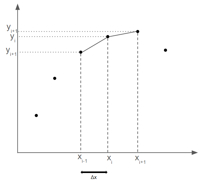
The finite difference method can be used whenever you have discrete data and you need to approximate an nth order derivative. An example follows. Suppose we are given arrays x and y (and do not know the function relating y to x), and we want to solve for the second derivative $ \frac{d^2y}{dx^2}$
import numpy as np
x= np.array([0,1,2,3,4,5,6,7,8,9,10])
y= 2*x**4+2
deltax= x[1]-x[0]
import matplotlib.pyplot as plt
plt.scatter(x,y)
plt.show()

We create an array to store our second derivative values. The central difference quotient only works for points with a neighbor on both sides, so we exclude the endpoints in our application of the equation.
Y= np.zeros(len(x))
for i in range(1,len(x)-1):
Y[i]=( y[i+1]-2*y[i]+y[i-1] )/ deltax
print(Y)
[ 0. 28. 100. 220. 388. 604. 868. 1180. 1540. 1948. 0.]
Since we chose a simple function for $y(x)$, we know that the 2nd derivative is $y'' = 24x^2$. Now we can compare our numerical solution to analytical.
Y_analytical= 24*x**2
plt.plot(x,Y,label= "finite difference")
plt.plot(x,Y_analytical, label="analytical")
plt.legend()
plt.title("Comparing the second derivative of y=2x^4+2")
plt.show()

In this simple case, apart from the endpoints, the numerical approximation is very close to true solution even with a large step size. With more complicated or rapidly changing functions, smaller step sizes are neded.
Finite Difference Method in our Project
The central difference method provides a second-order accurate approximation of the second derivative. It is given by: $$\frac{d^2 u_i}{dx^2} = \frac{u_{i-1}-2u_i+u_{i+1}}{(\Delta x)^2}$$ where $ \Delta x $ is the step size.
Finite difference method allows us to solve for the amplitude of the 2D plane over time by making approximations over small, finite spatial and time steps. Subsiting the second order derivatives in the wave equation with their finite difference counterpart yields: $$ \frac{u_{i,j}^{n+1} - 2u_{i,j}^n + u_{i,j}^{n-1}}{\Delta t^2} = c^2 \left( \frac{u_{i+1,j}^n - 2u_{i,j}^n + u_{i-1,j}^n}{\Delta y^2} + \frac{u_{i,j+1}^n - 2u_{i,j}^n + u_{i,j-1}^n}{\Delta x^2} \right) $$
If we rearange this equation, we can solve for the amplitude at the next time step:
$$ u_{i,j}^{n+1} = 2u_{i,j}^n - u_{i,j}^{n-1} + c^2 \Delta t^2 \left( \frac{u_{i+1,j}^n - 2u_{i,j}^n + u_{i-1,j}^n}{\Delta x^2} + \frac{u_{i,j+1}^n - 2u_{i,j}^n + u_{i,j-1}^n}{\Delta y^2} \right)$$The Finite Difference Algorithm
Conceptual description of algorithm
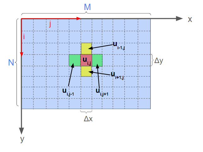
This code is intended to solve for the time evolution of a scalar waves in a rectangular two-dimensional region of space. The two-dimensional medium is disretized in to an NxM rectangular numpy array, of spatial resolution $\Delta x$ and $\Delta y$, with each spatial coordinate $(i,j)$ being assigned a scalar wave amplitude $u_{i,j}$. The second derivative with respect to x and y directions are approximated at each coordinate according to finite difference equation, using the neighbor coordinate amplitude values in the respective direction (Fig 1). The condition that the boundary of the 2D space have a fixed (zero) amplitude is applied by padding the initial amplitude array with a border whose values are 0.
At some time 0, we assume discrete knowledge of the amplitude and its first time derivative (i.e. amplitude velocity) on entire the 2D region. Since this algorithm treats velocity as the change in amplitude over discrete time steps, the velocity information is stored in the relative amplitudes of the first 2 time steps, which are provided as initial conditions. For conceptual convenience, a static intial amplitude configuration was assumed, as the behavior of wave oscillations from rest is more intuitive, and hence the physical fidelity of our model was easier to identify. However, alterations to the relative amplitudes of the initial two time steps would allow for the treatment of an arbitrary initial velocity.
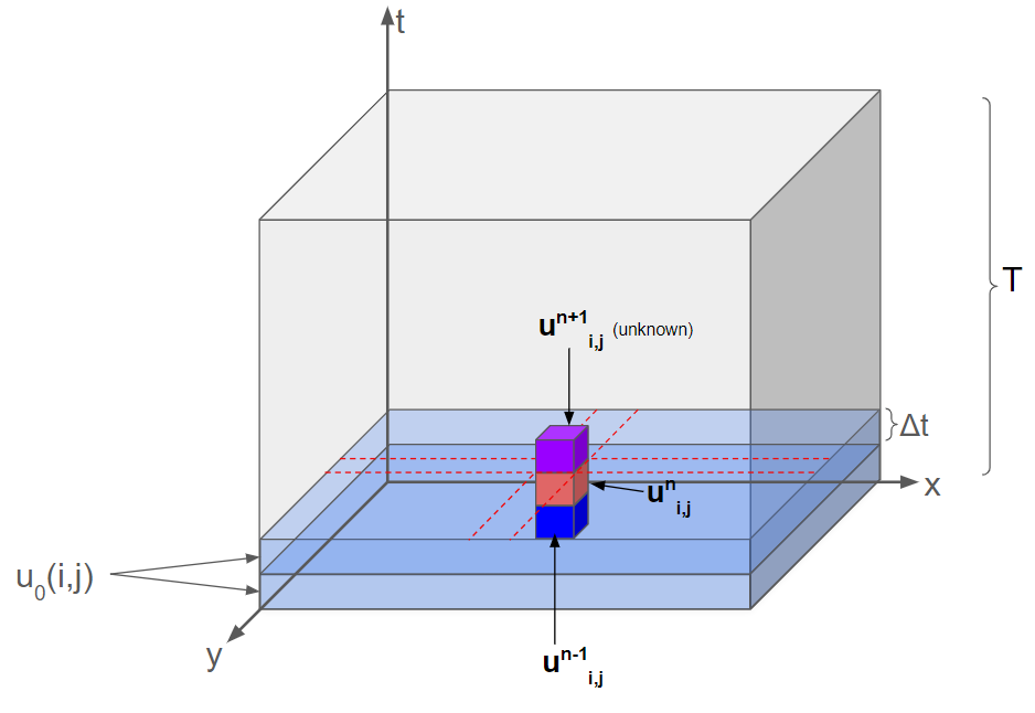
The full solution of the time evolution of this system can be described by a $N x M x T$ array, where $T$ is the total time of the simulation (Fig 2). The amplitude of the wave at a given coordinate in space and time $(i,j,n)$ is $u_{i,j}^n$. The first two layers in this 3D array are the two initial 2D amplitude arrays. The amplitude of time-neighbors of a particular coordinate are $u_{i,j}^{n-1}$ and $u_{i,j}^{n+1}$, where increasing $n$ denotes forward progress through time.
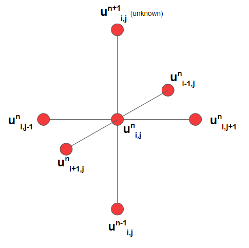
At a particular coordinate $(i,j)$, the amplitude of itself ($u_{i,j}^n$), its spatial neighbors ($u_{i,j-1}^n,u_{i,j+1}^n,u_{i-1,j}^n,u_{i+1,j}^n)$ and the previous time neighbor ($u_{i,j}^{n-1}$) are all known quantities. The equation for $u_{i,j}^{n+1}$ above solves for the forward time neighbor using the known amplitude values and the parameter for wavespeed, $c$. Figure 3 relates these quantities in stencil form. The algorithm performs this operation across all $(i,j)$ space coordinates and iterates forward in time until terminating after some specified amount of time steps. The resulting 3D array then contains all the information about the time evolution of the system.
The Script
As an example initial configuration, we choose a gaussian curve whose values depend on an equation, though the initial amplitude could be equally provided by discrete generated or measured data. Here, the initial 2D amplitude array (u_0_input) is created by performing numpy arithmetic with an X and Y meshgrid. The calculation and material parameters are also specified in the snippet below.
#importing python libraries
import numpy as np
import matplotlib.pyplot as plt
import matplotlib.animation as animation
from IPython.display import HTML
# Calculation parameters
M = 50 # 2D array width
N = 50 # 2D array height
deltat = 0.001 # time step
time_steps = 500 # total time steps
# Material parameters
c = 100 # material wave speed
# Create and populate initial 2D array with a Gaussian pulse
x = np.linspace(0, 10, M)
y = np.linspace(0, 10, N)
X, Y = np.meshgrid(x, y)
u_0_input = np.exp(-((X - 5) ** 2 + (Y - 5) ** 2))
# Define spatial resolution
deltax = x[1] - x[0]
deltay = y[1] - y[0]
The initial amplitude array has a border of thickness 1 appended to it using the $np.pad$.
All data for the solution is organized in a 3D numpy array, indexed with time, x coordinate, and y coordinate. In the snippet below, the array is initialized and its first two "slices of time" are populated with the two initial amplitude arrays.
# Pad array with boundary condition
u_0 = np.pad(u_0_input, pad_width=((1, 1), (1, 1)), mode='constant', constant_values=0)
# Create 3D array for storing all amplitude u data
Data = np.zeros((time_steps, N + 2, M + 2))
# Store initial amplitude for first two time steps
Data[0, :, :] = u_0
Data[1, :, :] = u_0
For all cells $(i,j)$ excluding the fixed boundary, the finite difference method equation is applied by looping over all i,j,n indices. The known and unknown amplitude values are acccessed and stored via indexing of the numpy array.
# Calculate d^2u/dx^2 and d^2u/dy^2 using finite difference method
for n in range(1, time_steps - 1):
for i in range(1, N + 1):
for j in range(1, M + 1):
Data[n + 1, i, j] = (
2 * Data[n, i, j]
- Data[n - 1, i, j]
+ (deltat ** 2 * c ** 2)
* ((Data[n, i + 1, j] - 2 * Data[n, i, j] + Data[n, i - 1, j]) / deltay ** 2
+ (Data[n, i, j + 1] - 2 * Data[n, i, j] + Data[n, i, j - 1]) / deltax ** 2))
To generate the animation for these simulations, we needed to use FuncAnimation. FuncAnimation takes a function, and calls it over a set of defined frames in order to generate an animation. Because we had already generated all of the data for each frame eariler using loops, we defined the animate function to go through that data and pull out each frame individually. In doing this, we stored each array into FuncAnimate and were able to display them as an animation.
Using the HTML plug-in, the animations were saved as videos.
# Create animation
fig, ax = plt.subplots(figsize=(8, 8))
im = ax.imshow(Data[0], cmap='viridis', interpolation='nearest', vmin=-1, vmax=1)
plt.colorbar(im, ax=ax)
def animate(i):
im.set_array(Data[i])
return [im]
ani = animation.FuncAnimation(fig, animate, frames=time_steps, interval=50, blit=True)
# Display animation in HTML
HTML(ani.to_jshtml())
Our first wave simulation was of a Gaussian pulse. This function is meant to simulate something akin to a raindrop, where there is a large perterbation in the center of a calm fluid. While damping is not being accounted for, we still get a model that behaves as expected. The wave travels radially outwards in all directions with the same velocity, and when it reaches a boundary, the polarity of the wave flips as it travels in a new direction
The next simulation is of a less symmetric initial amplitude, defined by a region of $u(x,y)=sin(xy)$. Due to the fixed boundary conditions, the dominant oscillations are those resulting from large magnitude initial amplitudes adjacent to the border. From our study of waves in paradigms, we expect large amplitude waves near a fixed boundary to change polarity and reflect. In a two dimensional rectangular region, this creates complicated patterns as the strong reflections reflect off the boundaries and interefere.
#Sine wave animation
import numpy as np
import matplotlib.pyplot as plt
import matplotlib.animation as animation
from IPython.display import HTML
# Material parameters
c = 100 # material wave speed
# Parameters
deltat = 0.0001 # time step
time_steps = 200 # total time steps
M = 50 # 2D array width
N = 50 # 2D array height
# Create and populate initial 2D array with sine wave function
x = np.linspace(1, 2, M)
y = np.linspace(2, 4, N)
u_0_input = np.zeros((N, M))
for i in range(N):
for j in range(M):
u_0_input[i, j] = np.sin(x[j] * y[i])
# Pad array with boundary condition
u_0 = np.pad(u_0_input, pad_width=((1, 1), (1, 1)), mode='constant', constant_values=0)
# Create 3D array for storing all amplitude u data
Data = np.zeros((time_steps, N + 2, M + 2))
# Store initial amplitude
Data[0, :, :] = u_0
Data[1, :, :] = u_0
# Define spatial steps
deltax = x[1] - x[0]
deltay = y[1] - y[0]
# Calculate d^2u/dx^2 and d^2u/dy^2 using finite difference method
for n in range(1, time_steps - 1):
for i in range(1, N + 1):
for j in range(1, M + 1):
Data[n + 1, i, j] = (
2 * Data[n, i, j]
- Data[n - 1, i, j]
+ (deltat ** 2 * c ** 2)
* ((Data[n, i + 1, j] - 2 * Data[n, i, j] + Data[n, i - 1, j]) / deltay ** 2
+ (Data[n, i, j + 1] - 2 * Data[n, i, j] + Data[n, i, j - 1]) / deltax ** 2))
# Create animation
fig, ax = plt.subplots(figsize=(8, 8))
im = ax.imshow(Data[0], cmap='viridis', interpolation='nearest', vmin=-1, vmax=1)
plt.colorbar(im, ax=ax)
def animate(i):
im.set_array(Data[i])
return [im]
ani = animation.FuncAnimation(fig, animate, frames=time_steps, interval=50, blit=True)
# Display animation in HTML
HTML(ani.to_jshtml())
We added a spatial-dependence for the wavespeed $c$, potentially useful for simulating wave propagation in non uniform mediums. For instance, sonar or seismic wave detection must take into account the varying mediums of their region of interest, due to varying salinity, pressure, temperature, rock composition, etc. Similarly, gradient-index optics manipulate the index of refraction of optical materials that can produce lenses with flat surfaces. Here, we define the spatially-dependent wavespeed with a numpy array that varies linearly with the $i$ coordinate (such as how wavespeed increases with depth below the surface in water). When simulating a symmetric waveform like the Gaussian curve, we notice that wavefront is distorted by the varying medium wavespeed, as the it travels much faster in the bottom of the frame compared to the top.
#Gaussian "raindrop" with spatially-dependent c
import numpy as np
import matplotlib.pyplot as plt
import matplotlib.animation as animation
from IPython.display import HTML
# Material parameters
c_cnst = 100 # material wave speed
# Parameters
deltat = 0.001 # time step
time_steps = 500 # total time steps
M = 50 # 2D array width
N = 50 # 2D array height
#Define spatial dependency of wavespeed (example)
c= np.ones((N+2,M+2))*c_cnst
for i in range(1,N):
c[i,:]= c_cnst*(i/N)+1
# Create and populate initial 2D array with a Gaussian pulse
x = np.linspace(0, 10, M)
y = np.linspace(0, 10, N)
X, Y = np.meshgrid(x, y)
u_0_input = np.exp(-((X - 5) ** 2 + (Y - 5) ** 2))
# Pad array with boundary condition
u_0 = np.pad(u_0_input, pad_width=((1, 1), (1, 1)), mode='constant', constant_values=0)
# Create 3D array for storing all amplitude u data
Data = np.zeros((time_steps, N + 2, M + 2))
# Store initial amplitude
Data[0, :, :] = u_0
Data[1, :, :] = u_0
# Define spatial steps
deltax = x[1] - x[0]
deltay = y[1] - y[0]
# Calculate d^2u/dx^2 and d^2u/dy^2 using finite difference method
for n in range(1, time_steps - 1):
for i in range(1, N + 1):
for j in range(1, M + 1):
Data[n + 1, i, j] = (2 * Data[n, i, j]- Data[n - 1, i, j]+ (deltat ** 2 * c[i,j] ** 2)
* ((Data[n, i + 1, j] - 2 * Data[n, i, j] + Data[n, i - 1, j]) / deltay ** 2
+ (Data[n, i, j + 1] - 2 * Data[n, i, j] + Data[n, i, j - 1]) / deltax ** 2))
# Create animation
fig, ax = plt.subplots(figsize=(8, 8))
im = ax.imshow(Data[0], cmap='bwr', interpolation='nearest', vmin=-1, vmax=1)
plt.colorbar(im, ax=ax)
def animate(i):
im.set_array(Data[i])
return [im]
ani = animation.FuncAnimation(fig, animate, frames=time_steps, interval=50, blit=True)
# Display animation in HTML
HTML(ani.to_jshtml())
Project Limitations
Some decisions taken limiting the scope of our model impose some restrictions on its accuracy in modelling real systems.
- This project does not take into account the dampening of waves
- Because this is a model of the non-dispersive wave equation, any limitations that equation may have will be reflected here as well.
- Our program only models waves and does not take into account more complicated fluid flow calculations, which makes for a less accurate model.
- Our project only applies to waves on square boundaries, which while a valid tool for simulations, does limit what scenarios can be modeled.
Intrinsic limitations
- Due to the way that our data is gathered, large wave speeds and time steps will result in data that is difficult, if not impossible, to interperet. Smaller wave speeds and time steps produce better results, which makes it difficult to model fast moving waves.
- No analytic solution to compare to for complicated systems: we are not sure our model is converged.
Display
- While not truly a limitation, the fact that our model is a simple heatmap and not a full 3D render does leave room for future improvements.
Coding Deep Dive: FuncAnimation (Student 2)
Introduction
What is FuncAnimation?
- FuncAnimation is a tool from the matplotlib library in Python, designed to create animations by repeatedly calling a function.
What is the Purpose of a FuncAnimation?
- Simply put, FuncAnimation exists to help coders in python create animations of different mathematical plots. These animations are frequently used to help visualize simulations.
When is it Appropriate to use FuncAnimation?
- FuncAnimation is best used when trying to display data that many need constant updating. This could be due to a function that is time dependent, or a live feed that needs to be frequently updated.
How To Use FuncAnimation
Function Syntax
To help explain the syntax of FuncAnimation, lets first start with a basic representation of FuncAnimation:
import matplotlib.animation as animation
ani = animation.FuncAnimation(fig, update, frames=, init_func=, interval=, blit=)
- Because animation is built into matplotlib, it first must be imported into python and defined in order to work
- "fig" is the figure object on which the animation will be drawn, and contains all the subplots and graphical elements that comprise the plot.
- "update" is the function that will be called at each frame of the animation
- "frames" parameter specifies the number of frames in the animation.
- "init_func" is whay will display on the first frame of the animation.
- "interval" controls the delay between frames in milliseconds.
- "blit" controls whether blitting is used to optimize the drawing of the animation. Blitting is a technique that redraws only the parts of the plot that have changed since the last frame, improving performance
Each of the above inputs will either require a numerical input, or an input that corresponds to a something that has been explictly defined, like a figure or a function.
Now, lets look at a simple example FuncAnimation to help further our understanding of them:
Worked Example - 1D Sine Wave Time Evolution
In this situation, you want to model a sine wave as time evolves. By using FuncAnimation, this process is relatively simple.
import numpy as np
import matplotlib.pyplot as plt
from matplotlib.animation import FuncAnimation
from IPython.display import HTML
First, we want to import all of the important plug-ins that we will be using. For the most part, these should seem familar, save for two exceptions. The "from IPython.display import HTML" command line is used to display our animation as an HTML. Jupyterhub can struggle with animations, and displaying them as an HTML in the notebook circumvents these issues. The "%matplotlib inline" command line does not import anything, but is simply telling Jupyterhub to embed the following animation inside the notebook.
fig, ax = plt.subplots()
xdata = np.linspace(0, 2 * np.pi, 100)
ydata = np.sin(xdata)
line, = ax.plot(xdata, ydata)
ax.set_xlim(0, 2 * np.pi)
ax.set_ylim(-1, 1)
(-1.0, 1.0)
This block of code is setting up our figure and the intial data for the sine function. This is where the first input into our FuncAnimate is defined. The "fig" is defined by our two limts for the axes.
def init():
line.set_ydata(np.sin(xdata))
return line,
Here, the intial frame of the animation is defined, which is another one of the inputs needed.
def update(frames):
line.set_ydata(np.sin(xdata + 0.1 * frames))
return line,
This code is defining the "update" input for FuncAnimation. Every frame of the animation, the phase is shfited by 0.1, which is essentially a time evolution.
ani = FuncAnimation(fig, update, frames=100, init_func=init, interval=50, blit=True)
HTML(ani.to_jshtml())
Finally, we have the FuncAnimation function itself. The remaining inputs, like the interval, frame, and blit are set to values so that the animation will display smoothly and for a reasonable amount of time.
FuncAnimation in Our Project
Our project used FuncAnimation extensively to achieve the animated plots of our 2D waves:
import numpy as np
import matplotlib.pyplot as plt
import matplotlib.animation as animation
from IPython.display import HTML
# Material parameters
c = 100 # material wave speed
# Parameters
deltat = 0.001 # time step
time_steps = 500 # total time steps
M = 50 # 2D array width
N = 50 # 2D array height
# Create and populate initial 2D array with a Gaussian pulse
x = np.linspace(0, 10, M)
y = np.linspace(0, 10, N)
X, Y = np.meshgrid(x, y)
u_0_input = np.exp(-((X - 5) ** 2 + (Y - 5) ** 2))
# Pad array with boundary condition
u_0 = np.pad(u_0_input, pad_width=((1, 1), (1, 1)), mode='constant', constant_values=0)
# Create 3D array for storing all amplitude u data
Data = np.zeros((time_steps, N + 2, M + 2))
# Store initial amplitude
Data[0, :, :] = u_0
Data[1, :, :] = u_0
# Define spatial steps
deltax = x[1] - x[0]
deltay = y[1] - y[0]
# Calculate d^2u/dx^2 and d^2u/dy^2 using finite difference method
for n in range(1, time_steps - 1):
for i in range(1, N + 1):
for j in range(1, M + 1):
Data[n + 1, i, j] = (2 * Data[n, i, j]- Data[n - 1, i, j]+(deltat ** 2 * c ** 2)*((Data[n, i + 1, j] - 2 * Data[n, i, j] + Data[n, i - 1, j]) / deltay ** 2+ (Data[n, i, j + 1] - 2 * Data[n, i, j] + Data[n, i, j - 1]) / deltax ** 2))
# Create animation
fig, ax = plt.subplots(figsize=(8, 8))
im = ax.imshow(Data[0], cmap='viridis', interpolation='nearest', vmin=-1, vmax=1)
plt.colorbar(im, ax=ax)
def animate(i):
im.set_array(Data[i])
return [im]
ani = animation.FuncAnimation(fig, animate, frames=time_steps, interval=50, blit=True)
# Display animation in HTML
HTML(ani.to_jshtml())
Lets break this down to see how FuncAnimate was used:
import numpy as np
import matplotlib.pyplot as plt
import matplotlib.animation as animation
from IPython.display import HTML
Here, we have the imporant plug-ins being imported into our notebook. This includes and defines how we will be calling animations from matplotlib.
deltat = 0.001 # time step
time_steps = 500 # total time steps
M = 50 # 2D array width
N = 50 # 2D array height
The "time_steps" varible is what we are using to determine the number of frames we will be including in our animation. This way, we get an animation that includes every piece of data that we generate.
fig, ax = plt.subplots(figsize=(8, 8))
im = ax.imshow(Data[0], cmap='viridis', interpolation='nearest', vmin=-1, vmax=1)
plt.colorbar(im, ax=ax)
<matplotlib.colorbar.Colorbar at 0x12c29f290>
In this chunk of code, we first define a figure and its size. Then, we do a step that is a bit more complicated. The ax.imshow function displays data as an image inside of a figure. We first need to define how our images will generate inside of the figure because we are going to be using FuncAnimate without a true function to plot.
for n in range(1, time_steps - 1):
for i in range(1, N + 1):
for j in range(1, M + 1):
Data[n + 1, i, j] = (2 * Data[n, i, j]- Data[n - 1, i, j]+(deltat ** 2 * c ** 2)*((Data[n, i + 1, j] - 2 * Data[n, i, j] + Data[n, i - 1, j]) / deltay ** 2+ (Data[n, i, j + 1] - 2 * Data[n, i, j] + Data[n, i, j - 1]) / deltax ** 2))
As you can see, we don't have a function that calculates the wave function for us. Instead, we are using a loop to calculate the wavefunction at every time step. By first defining "im" as the first time step of the wave function calculation, we can make a sudo-function.
def animate(i):
im.set_array(Data[i])
return [im]
We use "animate" to create our sudo-function. "animate" works by updating the im.show() varible at each time step. This collects all of the wavefunction calculations and allows us to display them using FuncAnimate.
ani = animation.FuncAnimation(fig, animate, frames=time_steps, interval=50, blit=True)
# Display animation in HTML
HTML(ani.to_jshtml())
Finally, we reach FuncAnimation itself. All of the varibles have been defined, and we use the HTML plug in to display our animation as a video